Building a Wiley Manuscript with Per-Chapter Bibliographies

One of Tech’s faculty and a post-doctoral research associate are working on a book for Wiley, and they want to have a list of references after each chapter, rather than one set of references for the entire book. Wiley’s LaTeX guides don’t give particularly good information on how to do this, and I never got a response back from the Wiley documentclass author on how best to handle this. So, in the interests of anyone searching for this in the future, here’s what I came up with.

Procedure:

  1. Pick the appopriate script for your operating system. There’s one script for Windows users, and another for Unix and OS X users.
  2. Edit the script to match your main filename (without the .tex extension). In my example, my main file was w-bksamp-minimal.tex, so I used w-bksamp-minimal.
  3. Rename your chapter content so each filename starts with “chapter-” — if you don’t like that restriction, feel free to edit the script to your liking.
  4. Make sure you use \include instead of \input to add each chapter to your main .tex file. Using \input will put multiple chapters’ citations into one .aux file, and BibTeX won’t be able to tell which bibliography entries go with each chapter.
  5. Adjust the latex, dvips, and ps2pdf lines to match your build process. I normally don’t use dvi at all, but I didn’t want to disrupt the Wiley procedures by default.

Windows version (attached as wiley-build-windows.zip)

@echo off
rem wiley-build.cmd -- Mike Renfro <renfro@tntech.edu>, 2011/11/06
rem
rem Cleaner build procedure for Wiley's wileySix and wileySeven
rem document classes that allows for per-chapter bibliographies
rem generated with BibTeX.

rem Instructions:
rem 1. Replace w-bksamp-minimal with the filename of the main .tex file
set mainfile=w-bksamp-minimal
rem 2. Rename each chapter to start with chapter- (for example:
rem    chapter-1.tex, chapter-mimo.tex, etc.)
rem 3. Make sure to use \include for each chapter in the main .tex file,
rem    not \input.

rem Should be no need to edit anything below this line.
latex %mainfile%
echo ...
for %%c in (chapter-*.tex) do bibtex %%~nc%
echo ...
latex %mainfile%
latex %mainfile%
dvips %mainfile%.dvi
ps2pdf %mainfile%.ps
rem Procedure adapted from
rem http://tex.stackexchange.com/questions/17474/multiple-bibliographies

Unix and OS X version (attached as wiley-build-unix-osx.zip)

#!/bin/sh

# wiley-build.sh -- Mike Renfro <renfro@tntech.edu>, 2011/11/06
#
# Cleaner build procedure for Wiley's wileySix and wileySeven
# document classes that allows for per-chapter bibliographies
# generated with BibTeX.

# Instructions:
# 1. Replace w-bksamp-minimal with the filename of the main .tex file
mainfile=w-bksamp-minimal
# 2. Rename each chapter to start with chapter- (for example:
#    chapter-1.tex, chapter-mimo.tex, etc.)
# 3. Make sure to use \include for each chapter in the main .tex file,
#    not \input.

# Should be no need to edit anything below this line.
latex ${mainfile}
echo ...
for c in chapter-*.tex; do
    bibtex `basename ${c}`
done
echo ...
latex ${mainfile}
latex ${mainfile}
dvips ${mainfile}.dvi
ps2pdf ${mainfile}.ps
# Procedure adapted from
# http://tex.stackexchange.com/questions/17474/multiple-bibliographies
OCR of scanned pages on Ubuntu 10.04

Just for future reference:

  1. Scan images at 300 dpi (might be able to make this work at a lower resolution, but this is fine). For one sample page, this resulted in a 2348×3129 pixel image where each baseline height was around 50 pixels, and capital letters had a height around 30 pixels.
  2. Install ocropus 0.3.1-2 from Ubuntu mirror. Other Ubuntu versions may have other ocropus versions.
  3. Run
    ocroscript recognize image.png > image.html

One More Update to the Door Sign Javascript

One more set of bug fixes for this original post.

Sometime early this week, Twitter broke some redirection I had been relying on. That is, if I was on my phone, URLs on twitter.com automatically redirected to mobile.twitter.com and kept all my parameters for status and such. mobile.twitter.com had no problem handling the request if I went there explicitly, though.

So here’s the code that lets the phone automatically run to the mobile site, and keeps the PC on the regular site. Yes, it’s browser detection and not feature detection, but I’m the only user, and anyone else wanting to do this kind of thing will probably be similarly relaxed on requirements.

Continue reading “One More Update to the Door Sign Javascript”

Updated HTML and Python code for Tweetable Office Door Sign

See the original post for the basic information. This post exists only to highlight a few bug fixes.

Since running with my sign for a few days, the main bug I’ve run into is that Twitter doesn’t let you post identical status messages over a short period of time. One recommended fix is to append some sort of unique data to each message. So I’ve decided to

  1. Convince my browser to append a millisecond time value to each message, and enclose the value in curly braces. So a status message of “In office” becomes “In office {339}”, for example.
  2. Modify the Python script to strip out the millisecond value so it doesn’t show up on the door sign. We’ll use a regular expression to filter out any pair of curly braces surrounding 1-3 digits.

Updated code is below the break.

Continue reading “Updated HTML and Python code for Tweetable Office Door Sign”

Work in Progress: Tweetable Office Door Sign

A sizable amount of my work week is spent outside of my office, and is difficult to schedule ahead of time:

  • Material testing jobs show up with little notice.
  • Students or faculty need help fixing a coding, instrumentation, or other problem, and it’s easiest to fix those on-site rather than in my office.
  • etc.

I’ve got a spot on my door for a 3×5 index card where I can post my known schedule (classes, regular meetings, that sort of thing), but I’ve always had to keep a stack of Post-It notes on hand for the other places I often go. The problem with the Post-It method is that I’ll often get called off to another location before I can get back to my office, and the notes quickly become inaccurate. And the notes can easily get misplaced or out of order, making them less useful.

And I liked the concept of the Panic Status Board, too.

So what I’m working on instead is a door sign I can update over the network from my smartphone, my home or office PC, someone else’s computer, etc. My office door already has a 12 inch square window in it, so any display I mount there can be protected, at least when the door is closed. There are several ways I could do this with varying tradeoffs:

  • YBox2 plus LCD TV and Twitter feed. Pros: would work out of the box for $150 in hardware costs and a bit of assembly and soldering. Cons: without modifying the Twitter widget code, I’d have to worry about the risk of someone else switching my door sign to another Twitter user, or else put the YBox2 on an isolated and firewalled network segment. And I’d have to either learn soldering or beg someone else to put it together for me.
  • Two XBee modules, one USB adapter, one compatible character LCD screen, and an always-on computer (probably my Mac Mini, since my main office PC is an often-mobile laptop). Pros: all the customization I’d ever want. Cons: all the customization I’d never want to implement. And more soldering.
  • Arduino, Ethernet shield, and firmware to parse an RSS or Twitter feed. Pros: probably easier to customize the firmware than the YBox2. Cons: $100 or more in hardware.
  • #twatch as an LCD Smartie display. Pros: super-cheap at $40 assembled. Cons: needing LCD Smartie to run on OS X, plus needing an extra network interface for the Mini.
  • Chumby or other Internet-connected display device. Pros: cheap, especially the $50 Insignia-branded one at Best Buy. Wifi built in. Cons: customization limited to whatever widgets people have already posted, or to my ability to code my own Flash widgets.


I ended up buying an Insignia Chumby because for $50, even if I just made it into a smarter alarm clock with MP3 and FM radio playback, it’d be an improvement over my current home clock. But I think it’ll end up working out well for my door sign. The setup details follow after the jump:
Continue reading “Work in Progress: Tweetable Office Door Sign”

Power Law Curve Fits in MATLAB

(See this Wikipedia article for a quick review of Power law fits.)

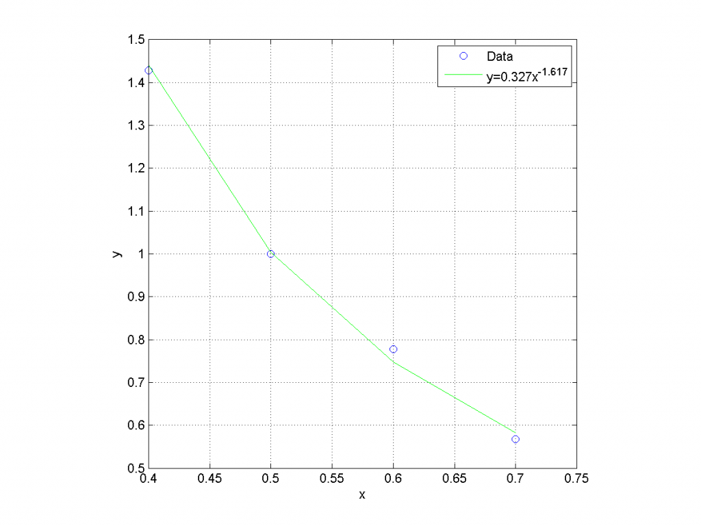
So linear curve fits are easy in MATLAB — just use p=polyfit(x,y,1), and p(1) will be the slope and p(2) will be the intercept. Power law fits are nearly as easy. Recall that any data conforming to a linear fit will fall along a given by the equation [latex]y=kx+a[/latex]
Similarly, any data conforming to a power law fit will fall along a curve given by the equation [latex]y=ax^k[/latex]
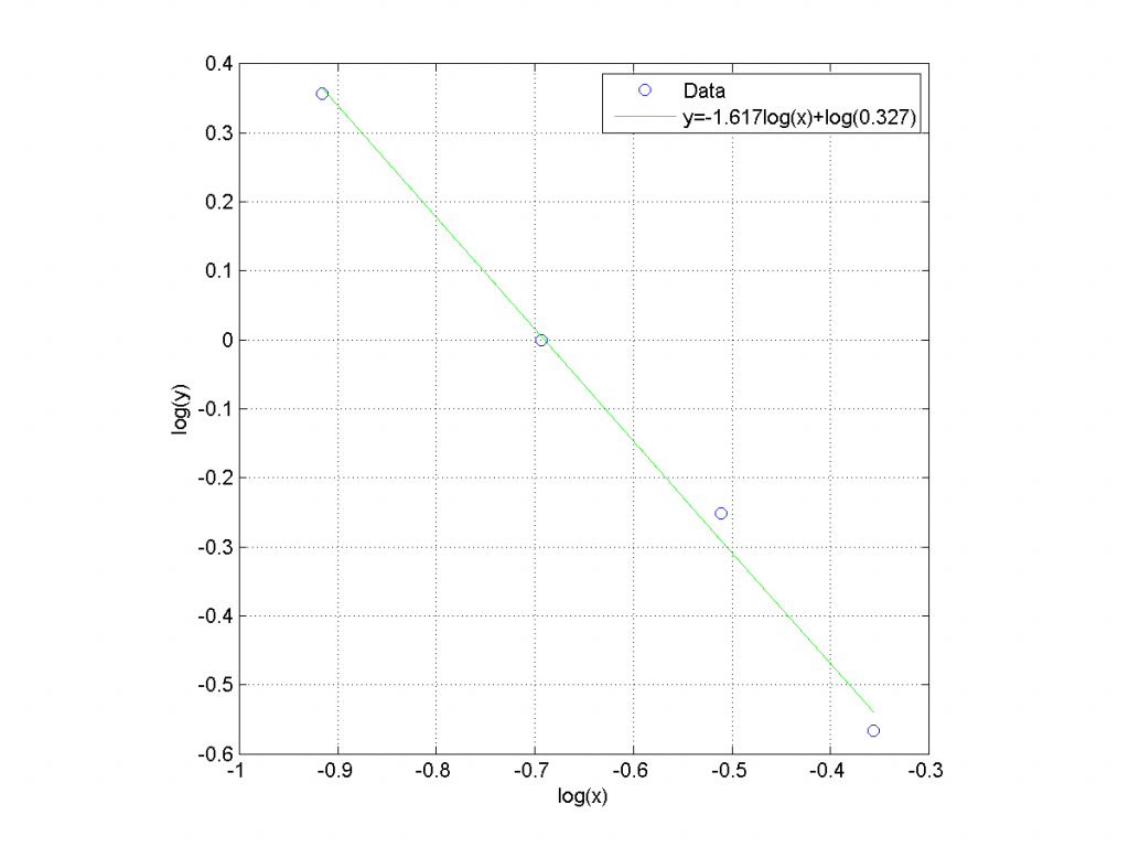
If we plot the second equation on log-log axes, it describes a family of straight lines. Put another way, if we take the log of y and x and plot them on linear axes, those logs will fall along a straight line. So all we need to do in MATLAB is to take the log of both x and y, and then let polyfit do its job. For example:

clear all
close all
x=[0.4 0.5 0.6 0.7];
y=[1.429 1 0.778 0.5675];
logx=log(x);
logy=log(y);
p=polyfit(logx,logy,1);
plot(logx,logy,'bo');
axis equal square
grid
xlabel('log(x)');
ylabel('log(y)');
k=p(1);
loga=p(2);
a=exp(loga);
hold on; plot(logx,k*logx+loga,'g')
legend('Data',sprintf('y=%.3f{}log(x)+log(%.3f)',k,a));
figure
plot(x,y,'bo');
xlabel('x');
ylabel('y');
axis equal square
grid
hold on; plot(x,a*x.^k,'g')
legend('Data',sprintf('y=%.3f{}x^{%.3f}',a,k));

returns the following figures:

fig1fig2

Nagios check_smb and Windows Server 2008R2

We’re in the midst of upgrading our Windows Server 2003 servers to 2008R2. Three down, one to go. We noticed that the 2008R2 servers threw errors back to Nagios that the 2003 servers never exhibited. Lots of:

CRITICAL SMB anon access: Domain=[CAE] OS=[Windows Server 2008 R2 Standard 7600] Server=[Windows Server 2008 R2 Standard 6.1]

errors. My obsessive-compulsive side finally got the best of me, and tonight I started digging into why these errors occur. The short form is that Server 2003 never cared if we had the wrong Netbios name when we queried it. Server 2008R2 (and possibly 2008 original) care greatly. To wit, on a Server 2003 target, these both work fine:

# /usr/lib/nagios/plugins/check_smb -H 149.149.254.IP1
OK Domain=[CAE] OS=[Windows Server 2003 3790 Service Pack 2] Server=[Windows Server 2003 5.2]
# /usr/lib/nagios/plugins/check_smb -H server2003.cae.tntech.edu
OK Domain=[CAE] OS=[Windows Server 2003 3790 Service Pack 2] Server=[Windows Server 2003 5.2]

but on a Server 2008R2 target, only the last one works:

# /usr/lib/nagios/plugins/check_smb -H 149.149.254.IP2
CRITICAL SMB anon access: Domain=[CAE] OS=[Windows Server 2008 R2 Standard 7600] Server=[Windows Server 2008 R2 Standard 6.1]
# /usr/lib/nagios/plugins/check_smb -H server2008r2.cae.tntech.edu
OK Domain=[CAE] OS=[Windows Server 2008 R2 Standard 7600] Server=[Windows Server 2008 R2 Standard 6.1]

check_smb takes its -H argument and passes it as the -L argument to smbclient (the Netbios name of the server you want to list shares on). So one quick change on my Nagios check_smb command from:

define command {
 command_name check_smb
 command_line /usr/lib/nagios/plugins/check_smb -H $HOSTADDRESS$
}

to

define command {
 command_name check_smb
 command_line /usr/lib/nagios/plugins/check_smb -H $HOSTNAME$
}

and everybody’s happy. I could have also changed check_smb to take both a $HOSTNAME$ and a $HOSTADDRESS$ argument to avoid problems if there’s a DNS failure, but this was the least invasive fix.

Using Matlab to Make Animations from Excel Simulation Results

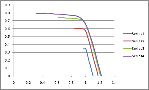
One of the faculty has some axisymmetric diffusion simulation code written in Excel and VBA. He didn’t think his 2D graphs of chemical concentration along a particle’s radius would be suitable for an audience he’d be presenting to, and that they’d be better served seeing an animation of how the concentration varied over time and position. Here’s where we started, more or less:

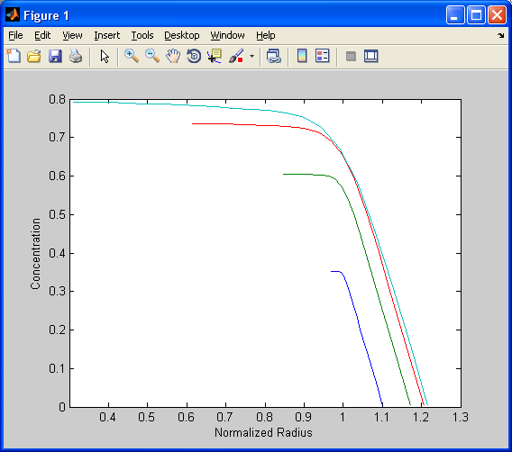
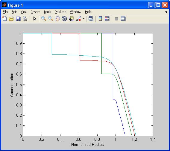
starting-point-exceland I had to be informed that the horizontal axis was radius from the particle center (normalized to 1 for the original particle radius), the vertical axis was something resembling a chemical concentration or composition, and that each line represented a different point in time. Excel’s default line thickness and other design choices bother me, so let’s go ahead and redo that graph in Matlab:starting-point-matlabAs it turns out, the concentration isn’t undefined closer to the particle center. Since this is a differential equation solution, we assume that the concentration is identically 1 everywhere from the center to the inside boundary radius. So, the total graphs of concentration versus distance should be:bc-addedwhich makes it a bit more explicit that we have a lump of pure material that gets gradually eaten away by its surroundings and becomes smaller.

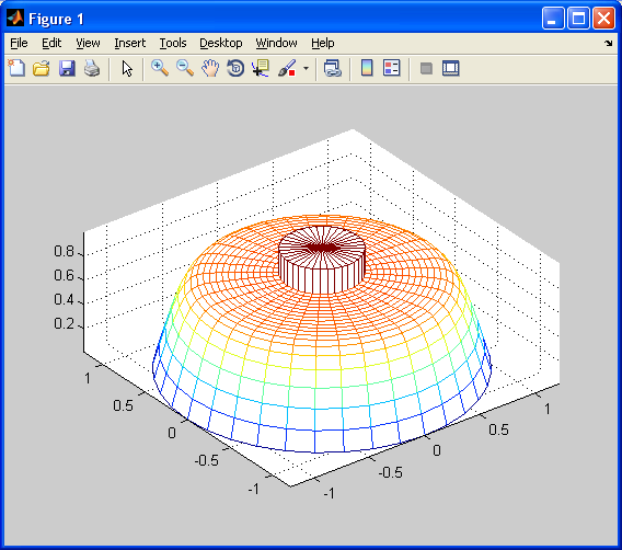
Now to convert that line graph into an axisymmetric representation. Mathworks already outlined how to do a basic mesh plot in polar coordinates, so all we have to do is adapt their instructions to our data. We don’t actually have to work out all the complex math, we just need to make a matrix for each point in time of equal size to the X and Y matrices created by meshgrid and pol2cart. Each column of this matrix should be the original Y data from Excel for that particular time, and the repmat function takes care of that. The resulting mesh plot of the last time step examined then looks like:mesh-frame-4All that’s left now is to:

  • Change the mesh plot to a surface
  • Remove the edge colors on each patch (so we have just the patch colors, not the edges)
  • Reorient our view to top-dead-center (like how we see the original material under the electron microscope)
  • Change the colormap to grayscale (like how we see the original material under the electron microscope)
  • Convert each plot into a frame of a video file with avifile and addframe.

Here’s the code:

clear all
close all
data=[ ...
    0.968682635	0.352941008	0.847944832	0.604846848	0.614770029	0.736745905	0.309963787	0.792192895
    0.975319116	0.352912882	0.864179809	0.60473259	0.644348798	0.736479267	0.355305164	0.791705755
    0.981955598	0.352843355	0.880414786	0.604508532	0.673927568	0.735967459	0.400646542	0.790820863
    0.988592079	0.352367206	0.896649763	0.604178754	0.703506337	0.735228449	0.445987919	0.789595717
    0.99522856	0.349314226	0.91288474	0.603743855	0.733085106	0.734277487	0.491329297	0.788068624
    1.001865042	0.339595849	0.929119717	0.603165414	0.762663875	0.733127586	0.536670674	0.786265735
    1.008501523	0.322069418	0.945354694	0.60215826	0.792242645	0.731789334	0.582012051	0.78420522
    1.015138005	0.300279218	0.961589671	0.599529003	0.821821414	0.730264749	0.627353429	0.781899808
    1.021774486	0.277475921	0.977824648	0.592185016	0.851400183	0.728502808	0.672694806	0.779357749
    1.028410967	0.254600132	0.994059625	0.575269388	0.880978952	0.726191443	0.718036184	0.776577069
    1.035047449	0.23173444	1.010294602	0.544925458	0.910557722	0.722114592	0.763377561	0.773500341
    1.04168393	0.208878058	1.026529579	0.501653986	0.940136491	0.712945073	0.808718939	0.76979412
    1.048320411	0.186029734	1.042764556	0.449999723	0.96971526	0.692373171	0.854060316	0.76410296
    1.054956893	0.163188804	1.058999533	0.394837376	0.999294029	0.652709252	0.899401693	0.752396638
    1.061593374	0.140354946	1.075234511	0.338837483	1.028872799	0.589603167	0.944743071	0.72609778
    1.068229856	0.117527765	1.091469488	0.282806787	1.058451568	0.505896949	0.990084448	0.672977986
    1.074866337	0.094706669	1.107704465	0.226853501	1.088030337	0.4097422	1.035425826	0.583653876
    1.081502818	0.071890988	1.123939442	0.170955144	1.117609106	0.308800318	1.080767203	0.459732008
    1.0881393	0.049079865	1.140174419	0.115095194	1.147187876	0.206932201	1.12610858	0.313724213
    1.094775781	0.026271856	1.156409396	0.059265944	1.176766645	0.10513866	1.171449958	0.159292943
    1.101412262	0.003483628	1.172644373	0.00345515	1.206345414	0.003440781	1.216791335	0.003438214
];
nFrames=size(data,2)/2; % due to 2 columns of data per frame
revgray=colormap(gray);
% 64x3 array of gray RGB values ([1 1 1] -> white and high values,
% [0 0 0] -> black and low values) -- gray is a built-in colormap
% revgray=revgray(size(revgray,1):-1:1,:);
% Reverse order of rows in revgray: results in a 64x3 array of gray RGB
% values ([0 0 0] -> black and high values, [1 1 1] -> white and low
% values)
fig=figure;
aviobj=avifile('diffusion.avi','FPS',15,'Quality',100);
for n=1:nFrames
    radius=data(:,n*2-1);
    concentration=data(:,n*2);
    % Add an extra data point at r=0 and r=min(r)
    radius=[0; min(radius); radius];
    concentration=[1; 1; concentration];
    % Build a polar grid (from Matlab help, "Displaying Contours in Polar
    % Coordinates")
    [th,r] = meshgrid((0:10:360)*pi/180,radius);
    [X,Y] = pol2cart(th,r);
    Z = X+i*Y; % For the purposes of polar math, abs(Z) is basically r.

    f=repmat(concentration,1,size(Z,2));
    % repmat(X,nr,nc) repeats X by nr rows and nc columns. size(Z,2)
    % returns the number of columns in Z. We end up with an array of
    % identical size to Z. f ends up being 1*concentration for all theta,
    % and concentration only varies with respect to r.

    surf(X,Y,abs(f),'EdgeColor','none');
    axis([-2 2 -2 2 0 1]);
    colormap(revgray);
    view(2);
    axis equal;
    title(sprintf('Frame %d',n));
    F=getframe(fig);
    aviobj=addframe(aviobj,F);
    pause(0.1);
end
aviobj=close(aviobj);

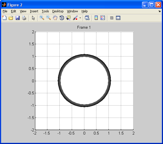
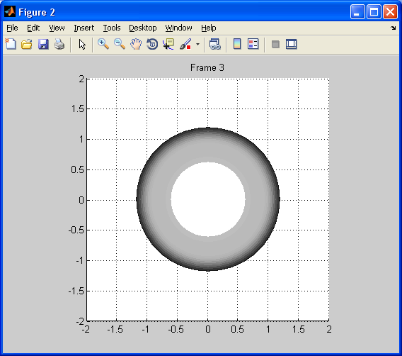
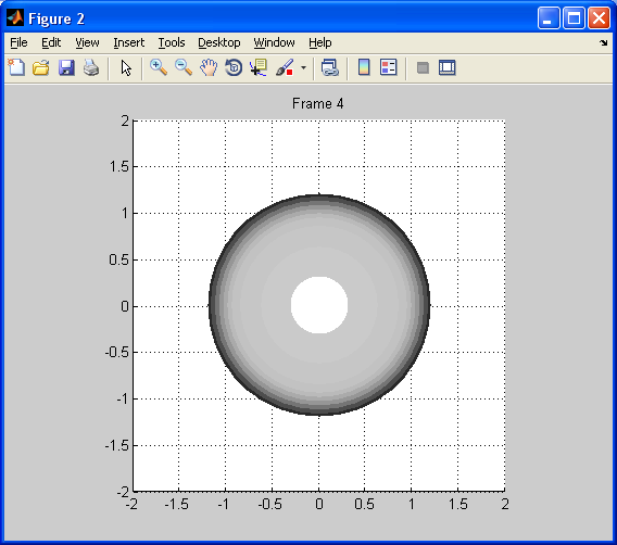
and the resulting still images and video:frame-1frame-2frame-3frame-4

Diffusion video (very short, 4 frames at 1 fps, may or may not play directly in the browser, so just download it)

Capturing an Image from a WIA-compatible Digital Camera

We’ve had a research project requiring a fair amount of image acquisition and processing, requiring  higher resolutions than most industrial cameras can offer. As a result, we’ve tried at least three different digital cameras (Canon PowerShot S3is, Nikon D40, and Canon PowerShot SD780is). Each of them has their own advantages and disadvantages:

  • S3is advantages:  good control with Breezesys’ PSRemote, including a pretty complete DLL that we can call from our LabVIEW code. Disadvantages: larger aperture sizes reduce the depth of field, and PSRemote can’t toggle macro and super-macro modes.
  • D40 advantages: complete manual control when needed, huge range of apertures including ones that allow for good depth of field, easy to grab pictures in PTP mode from Windows Explorer. Disadvantages: Breezesys’ NKRemote for Nikon doesn’t support the D40.
  • SD780is advantages: ridiculously high resolution (12MP) in a tiny camera. Disadvantages: no PSRemote support, and little manual control of settings.

So it came down to needing LabVIEW to acquire images from whatever camera automatically. We had gotten it working with PSRemote some time back for a different class of pictures, but the ones we needed now went beyond PSRemote’s and the S3is’ ability to focus in on close distances. And the SD780is was out entirely. So that left the Nikon.

Previous testing with the Nikon generally consisted of putting it in PTP mode, opening up Windows Explorer, hitting the “Take a new picture” link, and then copying over the newest image to the local drive. Great, except for the clicking and dragging. The obvious solution would be to automate the process via Win32 COM programming. After a few hours with the Python docs and MSDN, a workable Python script was born:

import win32com.client, time, os

WIA_COM = "WIA.CommonDialog"

WIA_DEVICE_UNSPECIFIED = 0
WIA_DEVICE_CAMERA = 2

WIA_INTENT_UNSPECIFIED = 0

WIA_BIAS_MIN_SIZE = 65536
WIA_BIAS_MAX_QUALITY = 131072

WIA_IMG_FORMAT_PNG = "{B96B3CAF-0728-11D3-9D7B-0000F81EF32E}"

WIA_COMMAND_TAKE_PICTURE="{AF933CAC-ACAD-11D2-A093-00C04F72DC3C}"

def acquire_image_wia():
    wia = win32com.client.Dispatch(WIA_COM) # wia is a CommonDialog object
    dev = wia.ShowSelectDevice()
    for command in dev.Commands:
        if command.CommandID==WIA_COMMAND_TAKE_PICTURE:
            foo=dev.ExecuteCommand(WIA_COMMAND_TAKE_PICTURE)

    i=1
    for item in dev.Items:
        if i==dev.Items.Count:
            image=item.Transfer(WIA_IMG_FORMAT_PNG)
            break
        i=i+1

    fname = 'wia-test.jpg'
    if os.path.exists(fname):
        os.remove(fname)
    image.SaveFile(fname)

os.chdir('c:/temp')
acquire_image_wia()

Things I like about this:

  • snaps the camera shutter, grabs the last image from the card, and stashes it on the local drive, no questions asked. Since I’ll probably set the camera settings once and leave it on manual focus, this is all I needed.
  • easily converted into an executable with py2exe.
  • roughly 3.2 seconds to acquire and save the image, with around 2 seconds of that spent on the ExecuteCommand() line with a 0.25 second shutter speed.

Things I don’t like about this:

  • Windows COM programming makes my brain hurt.
  • To make things entirely hands-off, I had to disable my Webcam. I’m sure there’s a way to make WIA connect to a named device, but ShowSelectDevice() was all I found ready documentation for. With multiple cameras available, it always asked which one I wanted to acquire from. With only one camera available, it just went on and snapped the picture.
  • I couldn’t find a good way of jumping to the end of the list of items stored on the camera. I can count them, I can iterate over them, but I’m having to iterate over each element until I get to the last one, and then I can transfer it over.

Someone may have a better solution to the last two problems, but this should get people started.

Update — Leaner, meaner code to grab the last image off one specified camera — thanks to Janzert in the comments below:

import win32com.client, time, os

MY_CAMERA="D40"
WIA_IMG_FORMAT_PNG = "{B96B3CAF-0728-11D3-9D7B-0000F81EF32E}"
WIA_COMMAND_TAKE_PICTURE="{AF933CAC-ACAD-11D2-A093-00C04F72DC3C}"

def acquire_image_wia():
    # Find the camera
    devman=win32com.client.Dispatch("WIA.DeviceManager")
    for info in devman.DeviceInfos:
        for prop in info.Properties:
            if prop.Name=="Name" and prop.Value==MY_CAMERA:
                dev = info.Connect()

    # Snap picture
    foo=dev.ExecuteCommand(WIA_COMMAND_TAKE_PICTURE)
    # Transfer last image (doesn't actually use PNG format, but this
    # still is valid syntax).
    image=dev.Items[dev.Items.count].Transfer(WIA_IMG_FORMAT_PNG)
    # Save into file
    fname = 'wia-test.jpg'
    if os.path.exists(fname):
        os.remove(fname)
    image.SaveFile(fname)

os.chdir('c:/temp')
acquire_image_wia()

Setting up Project Quotas under XFS in Debian GNU/Linux

Quick and dirty notes for getting XFS project quotas running: I’m working on making storage areas for various capstone design class groups, vehicle teams, etc. I’d like to ensure that they don’t take an excessive amount of storage, too. These instructions are slightly different than what I’d found elsewhere, and I’m hoping to have someone confirm that what I’m doing is correct and update the appropriate man pages accordingly.

So assuming we have a project for ME4444, group 3 (I already had projects defined for groups 1 and 2 from earlier tests):

# grep /home /etc/fstab
/dev/md1000/home        /home   xfs     defaults,usrquota,prjquota      0      1
# echo "me4444-03:/home/projects/me4444-03" >> /etc/projects
# echo "me4444-03:3" >> /etc/projid
# mkdir /home/projects/me4444-03
# xfs_quota -x -c "project -s me4444-03"
Setting up project me4444-03 (path /home/projects/me4444-03)...
Processed 1 /etc/projects paths for project me4444-03
# xfs_quota -x -c "limit -p bsoft=5g bhard=10g me4444-03"
# xfs_quota -x -c "report -p"
Project quota on /home (/dev/md1000/home)
                               Blocks
Project ID       Used       Soft       Hard    Warn/Grace
---------- --------------------------------------------------
me4444-01           0          0    1048576     00 [--------]
me4444-02           0    5242880   10485760     00 [--------]
me4444-03           0    5242880   10485760     00 [--------]

Now group 3 has a 5 GB “soft” quota, can exceed that for up to 7 days at a time, but can never exceed their 10 GB “hard” quota. All that’s left is setting up directory permissions and Samba configuration so that the authorized users can store things there.